Comprehensive Analysis for Laptop Prices & Model Building
Exploring Data Insights, Predictive Modelling and Interative Applications
1 OVERVIEW
In this mini project focused on laptop prices, a structured approach was employed, encompassing data cleaning, exploratory data analysis (EDA), feature engineering, regression model building, and the development of an interactive Shiny application. The data cleaning phase ensured the dataset’s integrity and usability, while EDA provided valuable insights into the characteristics and relationships within the dataset. Feature engineering enhanced the predictive capabilities of the model, leading to the development of a regression model to understand the determinants of laptop prices. The culmination of the project was the creation of an interactive Shiny application, allowing for dynamic exploration and visualization of the model’s predictions. This project serves as a comprehensive example of the end-to-end process of data analysis and model deployment, highlighting the multifaceted nature of predictive analytics in the realm of pricing.
2 INTRODUCTION
The mini project on laptop prices represents a comprehensive endeavor encompassing various stages of data analysis and model development. Beginning with data cleaning, the project involved meticulous preparation of the dataset to ensure its reliability and suitability for subsequent analysis. Following this, the exploratory data analysis (EDA) phase provided valuable insights into the characteristics and relationships within the dataset, laying the foundation for further exploration.Subsequently, feature engineering was carried out to enhance the predictive capabilities of the model, focusing on creating new features and transforming existing ones to improve its performance. The regression model building phase aimed to establish a predictive relationship between the features and the target variable, which in this case is laptop prices.The culmination of the project involved the development of an interactive Shiny application, enabling dynamic exploration and visualization of the model’s predictions. This interactive tool facilitated user engagement and provided a platform for gaining insights into the factors influencing laptop prices.Overall, this mini project serves as a demonstration of the end-to-end process of data analysis and model deployment, highlighting the multifaceted nature of predictive analytics in the context of pricing.
3 ABOUT DATASET
The dataset that is going to be used for various tasks of EDA is from Kaggle. The link to the dataset is attached below:
4 READING DATASET
5 DATA DESCRIPTION
The first 5 rows of the data
| company | type_name | inches | screen_resolution | cpu | ram | memory | gpu | op_sys | weight | price |
|---|---|---|---|---|---|---|---|---|---|---|
| Apple | Ultrabook | 13.3 | IPS Panel Retina Display 2560x1600 | Intel Core i5 2.3GHz | 8GB | 128GB SSD | Intel Iris Plus Graphics 640 | macOS | 1.37kg | 71378.68 |
| Apple | Ultrabook | 13.3 | 1440x900 | Intel Core i5 1.8GHz | 8GB | 128GB Flash Storage | Intel HD Graphics 6000 | macOS | 1.34kg | 47895.52 |
| HP | Notebook | 15.6 | Full HD 1920x1080 | Intel Core i5 7200U 2.5GHz | 8GB | 256GB SSD | Intel HD Graphics 620 | No OS | 1.86kg | 30636.00 |
| Apple | Ultrabook | 15.4 | IPS Panel Retina Display 2880x1800 | Intel Core i7 2.7GHz | 16GB | 512GB SSD | AMD Radeon Pro 455 | macOS | 1.83kg | 135195.34 |
| Apple | Ultrabook | 13.3 | IPS Panel Retina Display 2560x1600 | Intel Core i5 3.1GHz | 8GB | 256GB SSD | Intel Iris Plus Graphics 650 | macOS | 1.37kg | 96095.81 |
Column names of the dataset
Classes of dataset
'data.frame': 1303 obs. of 11 variables:
$ company : chr "Apple" "Apple" "HP" "Apple" ...
$ type_name : chr "Ultrabook" "Ultrabook" "Notebook" "Ultrabook" ...
$ inches : num 13.3 13.3 15.6 15.4 13.3 15.6 15.4 13.3 14 14 ...
$ screen_resolution: chr "IPS Panel Retina Display 2560x1600" "1440x900" "Full HD 1920x1080" "IPS Panel Retina Display 2880x1800" ...
$ cpu : chr "Intel Core i5 2.3GHz" "Intel Core i5 1.8GHz" "Intel Core i5 7200U 2.5GHz" "Intel Core i7 2.7GHz" ...
$ ram : chr "8GB" "8GB" "8GB" "16GB" ...
$ memory : chr "128GB SSD" "128GB Flash Storage" "256GB SSD" "512GB SSD" ...
$ gpu : chr "Intel Iris Plus Graphics 640" "Intel HD Graphics 6000" "Intel HD Graphics 620" "AMD Radeon Pro 455" ...
$ op_sys : chr "macOS" "macOS" "No OS" "macOS" ...
$ weight : chr "1.37kg" "1.34kg" "1.86kg" "1.83kg" ...
$ price : num 71379 47896 30636 135195 96096 ...- 9 character variables and 2 numeric variables
Variable Conversion
Converting variable names memory, weight & ram to be in numerical
Code
#variable conversion
library(dplyr)
laptop$ram=as.numeric(sub("GB","",laptop$ram))
laptop$weight=as.numeric(sub("kg","",laptop$weight))
laptop$memory=gsub("\\D","",laptop$memory) #removing words
laptop$memory=as.numeric(laptop$memory)
laptop$memory=ifelse(laptop$memory=="11",2000,laptop$memory)
laptop$memory=ifelse(laptop$memory=="2",2000,laptop$memory)
laptop$memory=ifelse(laptop$memory=="2561",1256,laptop$memory)
laptop$memory=ifelse(laptop$memory=="1281",1128,laptop$memory)
laptop$memory=ifelse(laptop$memory=="5121",1512,laptop$memory)
laptop$memory=ifelse(laptop$memory=="10",1000,laptop$memory)
laptop$memory=ifelse(laptop$memory=="2562",2256,laptop$memory)
laptop$memory=ifelse(laptop$memory=="5122",2512,laptop$memory)
laptop$memory=ifelse(laptop$memory=="1282",2128,laptop$memory)
laptop$memory=ifelse(laptop$memory=="256256",512,laptop$memory)
laptop$memory=ifelse(laptop$memory=="256500",756,laptop$memory)
laptop$memory=ifelse(laptop$memory=="25610",1256,laptop$memory)
laptop$memory=ifelse(laptop$memory=="51210",1512,laptop$memory)
laptop$memory=ifelse(laptop$memory=="512256",768,laptop$memory)
laptop$memory=ifelse(laptop$memory=="512512",1024,laptop$memory)
laptop$memory=ifelse(laptop$memory=="641",1064,laptop$memory)
laptop$memory=ifelse(laptop$memory=="1",1000,laptop$memory)
laptop %>%
dplyr::select(ram,weight,memory) %>% str()'data.frame': 1303 obs. of 3 variables:
$ ram : num 8 8 8 16 8 4 16 8 16 8 ...
$ weight: num 1.37 1.34 1.86 1.83 1.37 2.1 2.04 1.34 1.3 1.6 ...
$ memory: num 128 128 256 512 256 500 256 256 512 256 ...6 DATA CLEANING
Missing values
checking for any missing values in the dataset
| x | |
|---|---|
| company | 0 |
| type_name | 0 |
| inches | 0 |
| screen_resolution | 0 |
| cpu | 0 |
| ram | 0 |
| memory | 0 |
| gpu | 0 |
| op_sys | 0 |
| weight | 0 |
| price | 0 |
- no missing values
Duplicate entries
- no duplicated entries
7 VISUALIZATIONS & ANALYSIS
Code
library(ggplot2)
library(plotly)
library(tvthemes)
library(extrafont)
dt=laptop %>%
ggplot(aes(company,fill=type_name)) +
geom_bar(position = "dodge",width = 0.5) + theme_bw()+
theme(axis.text.x = element_text(size = 10, hjust=1,angle = 45))+
labs(title = "Distribution of Company vs Type of laptop ",
fill="Type of laptop",y="frequency")+
ggthemes::scale_fill_tableau()+
tvthemes::theme_avatar(text.font = "trebus ms") #distribution
ggplotly(dt)- Observation HP, Lenovo, Acer, Asus, Toshiba, Mediacom, Vero mostly produce Notebook laptops. Apple, Google, Microsoft mostly produces Ultra book laptops MSI and Razor mostly produces Gaming laptops
Skewness (Histogram/density plot)
Code
hist1=ggplot(laptop, aes=(x=price))+
geom_density(aes(x=price), stat = "density", fill="gold2",color="black")+
theme_bw()+labs(title = "Distribution of Price",
caption = "@Data Insights 2024") #density plot
hist2=ggplot(laptop,aes(x=price))+
geom_histogram(color="black",fill="gold2",stat = "bin")+
theme_bw()+labs(title = "Distribution of Price",y="frequency",
caption = "@Data Insights 2024")#histogram plot
hist1+
ggthemes::scale_fill_tableau()+
tvthemes::theme_brooklyn99(text.font = "trebuchet ms")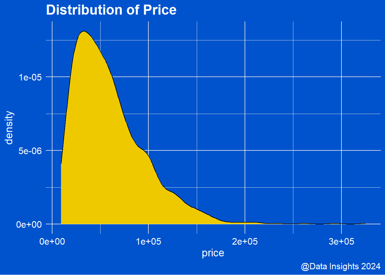
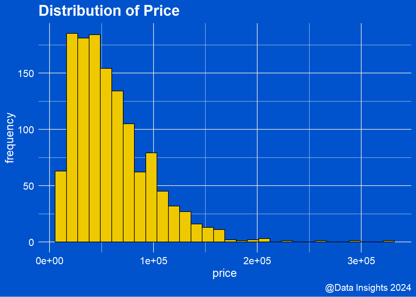
Observation
This shows that majority of laptops are concentrated on the lower end meaning that there are a very few laptops with high prices and a larger number of laptops with lower prices.
Brand name impact
Code
| Brand Name | Frequency |
|---|---|
| Dell | 297 |
| Lenovo | 297 |
| HP | 274 |
| Asus | 158 |
| Acer | 103 |
| MSI | 54 |
| Toshiba | 48 |
| Apple | 21 |
| Samsung | 9 |
| Mediacom | 7 |
| Razer | 7 |
| Microsoft | 6 |
| Vero | 4 |
| Xiaomi | 4 |
| Chuwi | 3 |
| Fujitsu | 3 |
| 3 | |
| LG | 3 |
| Huawei | 2 |
Observation
Major brand names in the market are dell, hp, acer, asus and lenovo
Expensive brand name in the market
Code
bn=ggplot(laptop, aes(x=company, y=price, fill=company))+
geom_boxplot(stat = "boxplot",outlier.color = "blue")+
theme(axis.text.x = element_text(size = 10, hjust=1,angle = 45))+
stat_summary(fun.y = median, geom = "point", shape=20, size=3, color="red")+
labs(y="average price",x="brand name",caption = "@Data Insights 2024")+
ggthemes::scale_fill_tableau()+
tvthemes::theme_avatar(text.font = "trebuchet ms",
text.size = 5)
ggplotly(bn)Observation
Razor is the most expensive as it has the highest average price
Popular Laptop type in the market
Code
| type of laptop | frequency |
|---|---|
| Notebook | 727 |
| Gaming | 205 |
| Ultrabook | 196 |
| 2 in 1 Convertible | 121 |
| Workstation | 29 |
| Netbook | 25 |
- Observation Notebooks, gaming, ultra book, 2 in 1 convertible are dominating in the market respectively
Most expensive type of laptops
Code
me=ggplot(laptop, aes(x=type_name, y=price, fill=type_name))+
geom_boxplot(stat = "boxplot")+
theme(legend.position ="right")+ theme_bw()+
theme(axis.text.x = element_text(size = 10, hjust=1,angle = 45))+
labs(fill="Laptop Type",y="average price",x="Laptop type",
caption = "@Data Insights 2024")
ggplotly(me)Observation
Workstations are more expensive.
Relationships (Scatter plots)
Relationship between the inches,memory,weight, ram and prices of laptops
Code
sp1=ggplot(laptop, aes(x=inches, y=price))+
geom_point(stat="identity",colour="orange",shape="circle")+
geom_smooth(method = "loess")+theme_linedraw()+
labs(caption = "@Data Insights 2024")+
tvthemes::theme_spongeBob(text.font = "trebuchet ms")
sp2=ggplot(laptop, aes(y=price,x=ram))+
geom_point(stat="identity",colour="red2",shape="triangle")+
geom_smooth(method = "loess")+theme_linedraw()+
labs(caption = "@Data Insights 2024")+
tvthemes::theme_hildaDusk(text.font = "trebuchet ms")
sp3=ggplot(laptop, aes(y=price,x=weight))+
geom_point(stat="identity",colour="green",shape="square")+
geom_smooth(method = "loess")+theme_linedraw()+
labs(caption = "@Data Insights 2024")+
ggthemes::scale_fill_tableau()+
tvthemes::theme_hildaNight(text.font = "trebuchet ms")
sp4=ggplot(laptop, aes(y=price,x=memory))+
geom_point(stat="identity",colour="blue4",shape="k")+
geom_smooth(method = "loess")+theme_linedraw()+
labs(caption = "@Data Insights 2024")+
ggthemes::scale_fill_tableau()+
tvthemes::theme_avatar(text.font = "trebuchet ms")
library(gridExtra)
grid.arrange(sp1,sp2,sp3,sp4,ncol=2,nrow=2)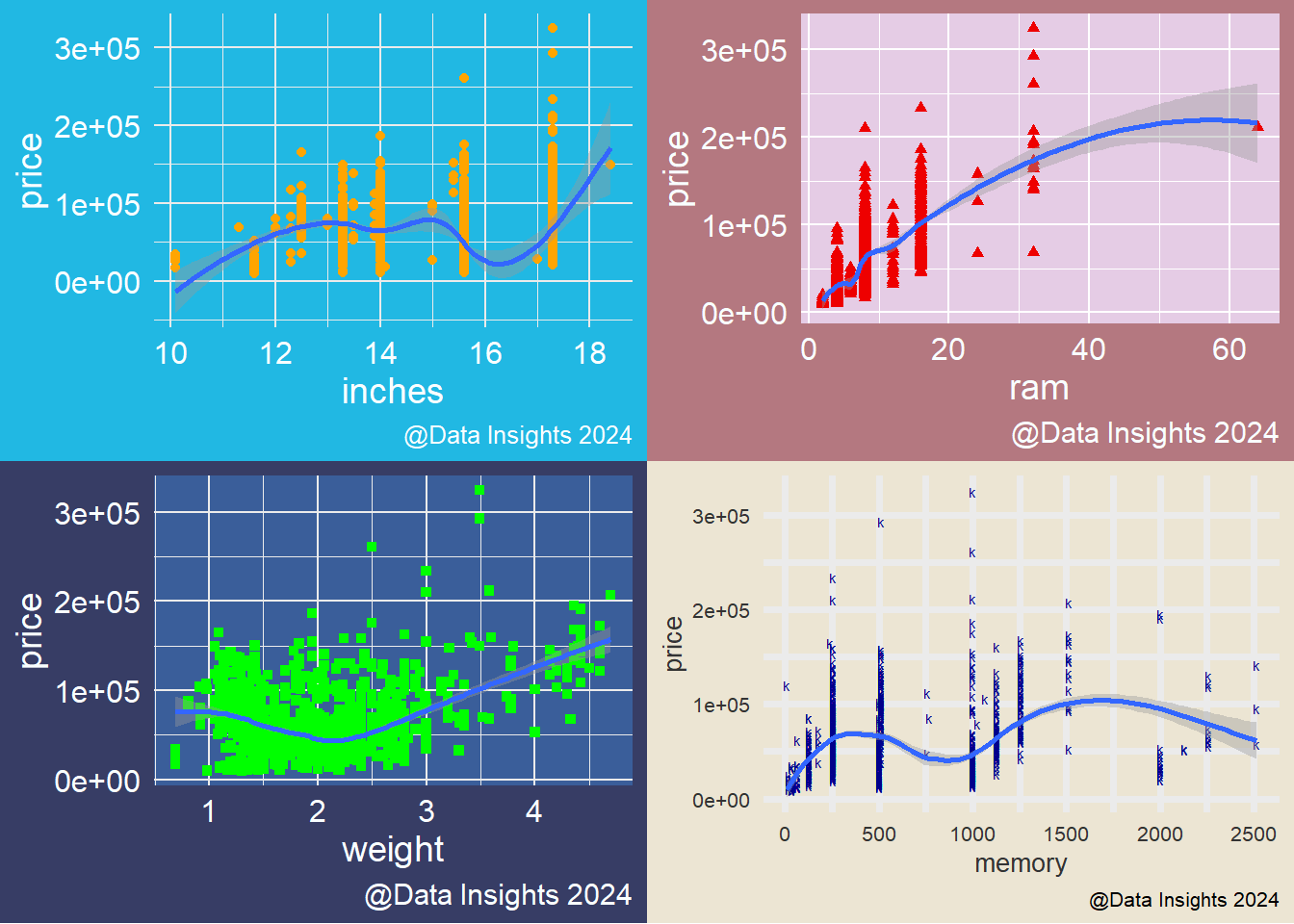
Observation
There is a relationship between the price of a laptop and it’s ram, memory,weight, inches.
As inches, ram, weight,memory increases, prices also increases
8 FEATURE ENGINEERING
1. SCREEN RESOLUTION
Adding New Columns (touchscreen,ips display,x & y dimensions,hd display)
Code
| Var1 | Freq |
|---|---|
| Full HD 1920x1080 | 507 |
| 1366x768 | 281 |
| IPS Panel Full HD 1920x1080 | 230 |
| IPS Panel Full HD / Touchscreen 1920x1080 | 53 |
| Full HD / Touchscreen 1920x1080 | 47 |
| 1600x900 | 23 |
| Touchscreen 1366x768 | 16 |
| Quad HD+ / Touchscreen 3200x1800 | 15 |
| IPS Panel 4K Ultra HD 3840x2160 | 12 |
| IPS Panel 4K Ultra HD / Touchscreen 3840x2160 | 11 |
- Top 10 rows of the screen resolution column
- The column is very noisy
Code
library(stringr)
result=as.data.frame(str_match(laptop$screen_resolution,"(\\d+)x(\\d+)"))
laptop=laptop %>%
mutate(x_dim=as.numeric(result$V2),
y_dim=as.numeric(result$V3))
laptop=laptop %>%
mutate(touchscreen=ifelse(grepl("Touchscreen",laptop$screen_resolution),1,0),
ips_display=ifelse(grepl("IPS Panel",screen_resolution),1,0),
hd_display=ifelse(grepl("Full HD",screen_resolution),1,0))
laptop %>%
dplyr::select(x_dim,y_dim,touchscreen,ips_display,hd_display) %>%
str()'data.frame': 1303 obs. of 5 variables:
$ x_dim : num 2560 1440 1920 2880 2560 ...
$ y_dim : num 1600 900 1080 1800 1600 768 1800 900 1080 1080 ...
$ touchscreen: num 0 0 0 0 0 0 0 0 0 0 ...
$ ips_display: num 1 0 0 1 1 0 1 0 0 1 ...
$ hd_display : num 0 0 1 0 0 0 0 0 1 1 ...- New dummy variables created
Touchscreen Feature
Code
| touchscreen feature | freq |
|---|---|
| 0 | 1111 |
| 1 | 192 |
Code
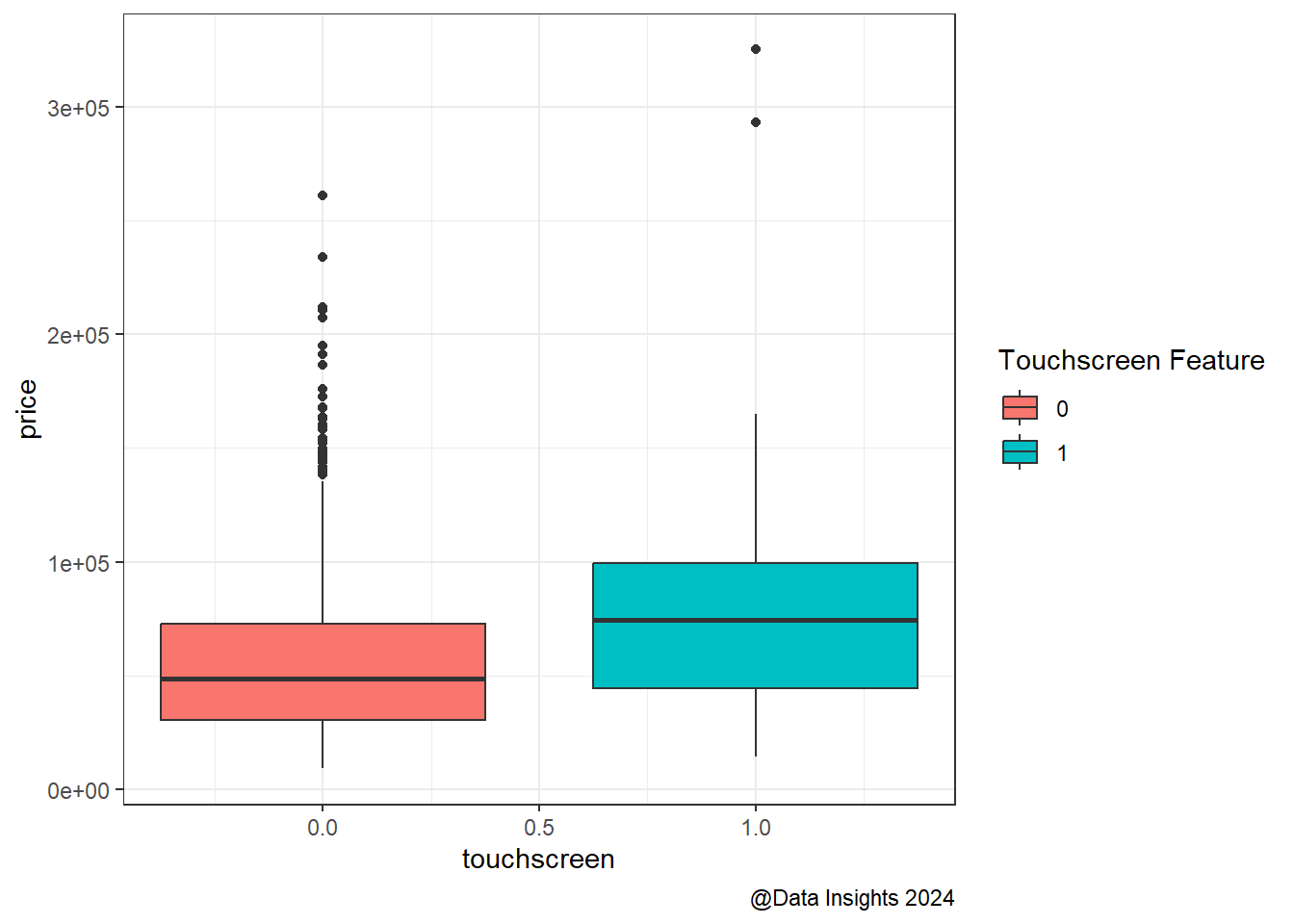
- Observation touchscreen=1 , non touchscreen=0 A few laptops have the touch screen feature Laptops with touchscreen features are more expensive
Ips Display Feature
Code
| ips display feature | freq |
|---|---|
| 0 | 938 |
| 1 | 365 |
Code
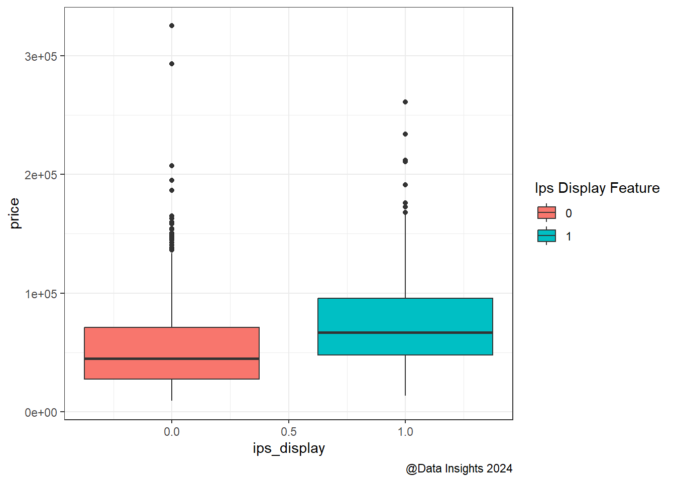
- Observation laptops with ips display=1 , laptops with non ips displays=0 365 laptops have ips display and 938 do not have ips display Laptops with ips display are more costly
HD Display Feature
Code
| hd display feature | freq |
|---|---|
| 0 | 460 |
| 1 | 843 |
Code
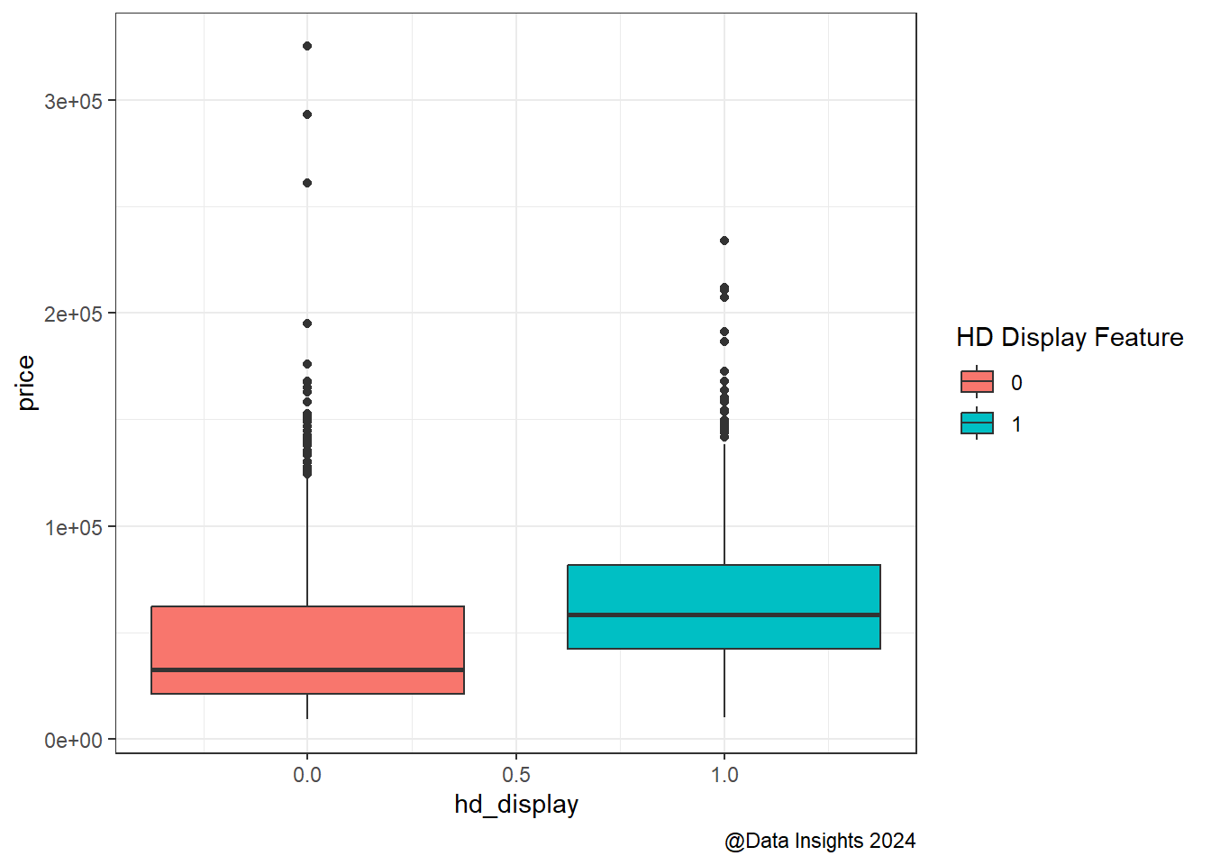
Observation
Hd display=1, non hd display=0
A lot of laptops have hd display
Laptops with hd display are more costly
Correlation
The new variables have to be in numeric format for correlation analysis
Code
| price | ips_display | hd_display | x_dim | y_dim | touchscreen | inches | weight | ram | memory | |
|---|---|---|---|---|---|---|---|---|---|---|
| price | 1.0000000 | 0.2522076 | 0.1986116 | 0.5565293 | 0.5528092 | 0.1912265 | 0.0681967 | 0.2103698 | 0.7430071 | 0.1608189 |
| ips_display | 0.2522076 | 1.0000000 | 0.1854415 | 0.2814567 | 0.2890295 | 0.1505123 | -0.1148042 | 0.0169671 | 0.2066225 | -0.0146866 |
| hd_display | 0.1986116 | 0.1854415 | 1.0000000 | 0.0708752 | 0.0486595 | -0.1051885 | 0.1635506 | 0.1480029 | 0.2103593 | 0.0903041 |
| x_dim | 0.5565293 | 0.2814567 | 0.0708752 | 1.0000000 | 0.9942190 | 0.3510657 | -0.0712453 | -0.0328798 | 0.4331205 | 0.0715309 |
| y_dim | 0.5528092 | 0.2890295 | 0.0486595 | 0.9942190 | 1.0000000 | 0.3579300 | -0.0954039 | -0.0538457 | 0.4244366 | 0.0569593 |
| touchscreen | 0.1912265 | 0.1505123 | -0.1051885 | 0.3510657 | 0.3579300 | 1.0000000 | -0.3617345 | -0.2946198 | 0.1169841 | -0.1384806 |
| inches | 0.0681967 | -0.1148042 | 0.1635506 | -0.0712453 | -0.0954039 | -0.3617345 | 1.0000000 | 0.8276311 | 0.2379928 | 0.5383581 |
| weight | 0.2103698 | 0.0169671 | 0.1480029 | -0.0328798 | -0.0538457 | -0.2946198 | 0.8276311 | 1.0000000 | 0.3838741 | 0.5497539 |
| ram | 0.7430071 | 0.2066225 | 0.2103593 | 0.4331205 | 0.4244366 | 0.1169841 | 0.2379928 | 0.3838741 | 1.0000000 | 0.3513626 |
| memory | 0.1608189 | -0.0146866 | 0.0903041 | 0.0715309 | 0.0569593 | -0.1384806 | 0.5383581 | 0.5497539 | 0.3513626 | 1.0000000 |
Observation
All the new variables created have a positive relationship with price x and y dimension have a strong positive relationship
Creating new variable called Pixel Per Inches (PPI) (getting rid of variables with low correlation)
Code
[1] 0.4734873- Improved correlation
2. CPU
Code
| . | Freq |
|---|---|
| Intel Core i5 7200U 2.5GHz | 190 |
| Intel Core i7 7700HQ 2.8GHz | 146 |
| Intel Core i7 7500U 2.7GHz | 134 |
| Intel Core i7 8550U 1.8GHz | 73 |
| Intel Core i5 8250U 1.6GHz | 72 |
| Intel Core i5 6200U 2.3GHz | 68 |
| Intel Core i3 6006U 2GHz | 64 |
| Intel Core i7 6500U 2.5GHz | 49 |
| Intel Core i7 6700HQ 2.6GHz | 43 |
| Intel Core i3 7100U 2.4GHz | 37 |
- Top 10 rows of the CPU column
- The column is noisy
Code
laptop=laptop %>%
mutate(intel_core_i3=ifelse(grepl("Intel Core i3",cpu),1,0),
intel_core_i5=ifelse(grepl("Intel Core i5",cpu),1,0),
intel_core_i7=ifelse(grepl("Intel Core i7",cpu),1,0),
dual_core=ifelse(grepl("Dual Core",cpu),1,0),
amd_processor=ifelse(grepl("AMD ",cpu),1,0),
other_processor=ifelse(grepl("Intel Xeon",cpu),1,0))
laptop %>% dplyr::select(intel_core_i3,intel_core_i5,intel_core_i7,dual_core,
amd_processor,other_processor) %>% str()'data.frame': 1303 obs. of 6 variables:
$ intel_core_i3 : num 0 0 0 0 0 0 0 0 0 0 ...
$ intel_core_i5 : num 1 1 1 0 1 0 0 1 0 1 ...
$ intel_core_i7 : num 0 0 0 1 0 0 1 0 1 0 ...
$ dual_core : num 0 0 0 0 0 0 0 0 0 0 ...
$ amd_processor : num 0 0 0 0 0 1 0 0 0 0 ...
$ other_processor: num 0 0 0 0 0 0 0 0 0 0 ...- New dummy variables created
3. GPU
| . | Freq |
|---|---|
| Intel HD Graphics 620 | 281 |
| Intel HD Graphics 520 | 185 |
| Intel UHD Graphics 620 | 68 |
| Nvidia GeForce GTX 1050 | 66 |
| Nvidia GeForce GTX 1060 | 48 |
| Nvidia GeForce 940MX | 43 |
| AMD Radeon 530 | 41 |
| Intel HD Graphics 500 | 39 |
| Intel HD Graphics 400 | 37 |
| Nvidia GeForce GTX 1070 | 30 |
- Top 10 rows of the Gpu column
- The column is very noisy
Code
'data.frame': 1303 obs. of 3 variables:
$ nvidia_graphics: num 0 0 0 0 0 0 0 0 1 0 ...
$ amd_graphics : num 0 0 0 1 0 1 0 0 0 0 ...
$ intel_graphics : num 1 1 1 0 1 0 1 1 0 1 ...- New dummy variables created
4. OP_SYS
Code
| . | Freq |
|---|---|
| Windows 10 | 1072 |
| No OS | 66 |
| Linux | 62 |
| Windows 7 | 45 |
| Chrome OS | 27 |
| macOS | 13 |
| Mac OS X | 8 |
| Windows 10 S | 8 |
| Android | 2 |
- Top 10 rows of the Op_sys column
- The column is very noisy
Code
laptop=laptop %>%
mutate(windows_10=ifelse(grepl("Windows 10",op_sys),1,0),
no_operating_system=ifelse(grepl("No OS",op_sys),1,0),
linux=ifelse(grepl("Linux",op_sys),1,0),
windows_7=ifelse(grepl("Windows 7",op_sys),1,0),
chrome_os=ifelse(grepl("Chrome OS ",op_sys),1,0),
mac_os=ifelse(grepl("macOS",op_sys),1,0),
mac_os_x=ifelse(grepl("Mac OS X",op_sys),1,0),
windows_10_s=ifelse(grepl("Windows 10 S",op_sys),1,0),
android=ifelse(grepl("Android",op_sys),1,0))
laptop %>%
dplyr::select(windows_10,no_operating_system,linux,windows_7,
chrome_os,mac_os,mac_os_x,windows_10,android)%>%str()'data.frame': 1303 obs. of 8 variables:
$ windows_10 : num 0 0 0 0 0 1 0 0 1 1 ...
$ no_operating_system: num 0 0 1 0 0 0 0 0 0 0 ...
$ linux : num 0 0 0 0 0 0 0 0 0 0 ...
$ windows_7 : num 0 0 0 0 0 0 0 0 0 0 ...
$ chrome_os : num 0 0 0 0 0 0 0 0 0 0 ...
$ mac_os : num 1 1 0 1 1 0 0 1 0 0 ...
$ mac_os_x : num 0 0 0 0 0 0 1 0 0 0 ...
$ android : num 0 0 0 0 0 0 0 0 0 0 ...- New dummy variables created
9 MODEL BUILDING (PREDICTING LAPTOP PRICE)
Multiple Linear Regression (Backward Approach)
Code
laptop_subset=laptop %>%
dplyr::select(6:7,10:11,14:35)
set.seed(1)
sample=sample(c(TRUE,FALSE),nrow(laptop_subset),replace=TRUE,prob = c(0.7,0.3))
train=laptop_subset[sample,]
test=laptop_subset[!sample,]
library(MASS)
full_model= lm(price ~ .,data = train)#full model including all the variables
output=capture.output(backward_regression<-
stepAIC(full_model,direction="backward",
scope=list(lower= ~1),
data=train)) #keeping significant variables
summary(backward_regression)
Call:
lm(formula = price ~ ram + memory + weight + hd_display + ppi +
intel_core_i3 + intel_core_i5 + intel_core_i7 + amd_processor +
other_processor + amd_graphics + no_operating_system + linux +
windows_7 + mac_os, data = train)
Residuals:
Min 1Q Median 3Q Max
-66745 -10935 -1733 8259 135827
Coefficients:
Estimate Std. Error t value Pr(>|t|)
(Intercept) -27256.725 4312.931 -6.320 4.13e-10 ***
ram 3630.263 180.835 20.075 < 2e-16 ***
memory -5.714 1.723 -3.315 0.000953 ***
weight 6531.871 1385.708 4.714 2.82e-06 ***
hd_display -2834.155 1523.850 -1.860 0.063233 .
ppi 211.398 19.225 10.996 < 2e-16 ***
intel_core_i3 7918.765 2824.250 2.804 0.005159 **
intel_core_i5 18141.763 2407.517 7.535 1.19e-13 ***
intel_core_i7 29296.716 2697.793 10.860 < 2e-16 ***
amd_processor 11233.685 4243.068 2.648 0.008251 **
other_processor 97142.568 14179.695 6.851 1.37e-11 ***
amd_graphics -11594.426 2336.324 -4.963 8.32e-07 ***
no_operating_system -13535.440 3352.309 -4.038 5.86e-05 ***
linux -9475.005 3244.385 -2.920 0.003583 **
windows_7 27642.342 3370.634 8.201 8.25e-16 ***
mac_os 10963.073 7525.384 1.457 0.145519
---
Signif. codes: 0 '***' 0.001 '**' 0.01 '*' 0.05 '.' 0.1 ' ' 1
Residual standard error: 19370 on 894 degrees of freedom
Multiple R-squared: 0.7348, Adjusted R-squared: 0.7304
F-statistic: 165.2 on 15 and 894 DF, p-value: < 2.2e-16Adjusted R Squared = 0.7304 means 73 percent of variance in the dependent variable (price) is explained by the independent variables hence it is a better fit of the model to the data.
P Value of 2.2e-16 <0.05 means that the model is statistical significant in predicting the price of a laptop.
Assumptions of Multiple Linear Regression
1. Linearity of the relationship
Code
- There is no pattern hence assumption not violated
2. Independence of errors
lag Autocorrelation D-W Statistic p-value
1 0.0472467 1.90477 0.14
Alternative hypothesis: rho != 0- D-W statistic close to 2 indicates no auto correlation (1.90477 is approximately 2) hence assumption not violated
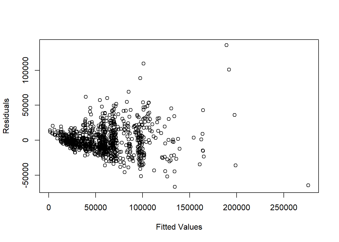
3. Homoscedacity (Constant Variance of Residuals)
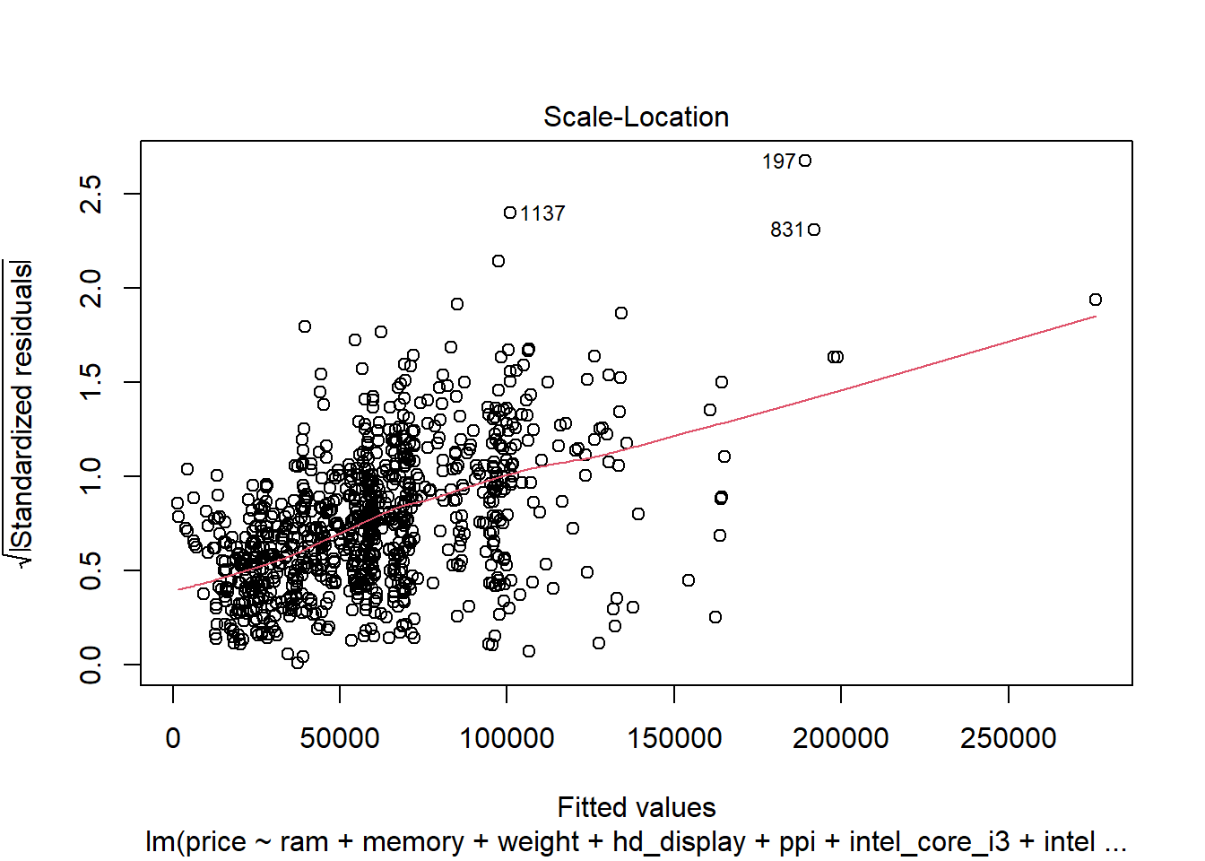
- No cone shaped pattern hence assumption not violated
4. Normality of Residuals
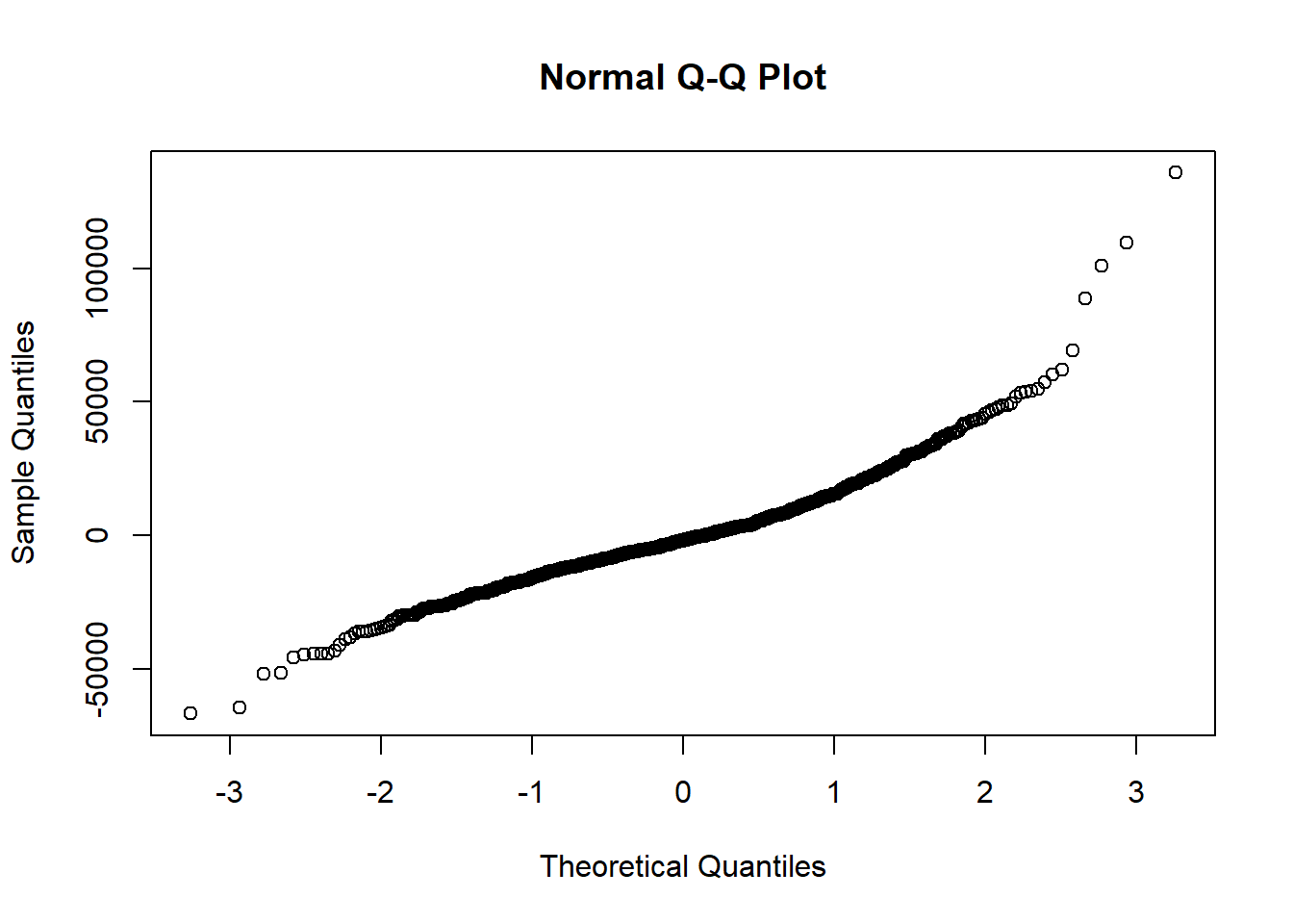
- No deviations from normality hence assumption not violated
5. Multicollinearity
ram memory weight hd_display
1.981195 1.548162 1.986819 1.285926
ppi intel_core_i3 intel_core_i5 intel_core_i7
1.580429 1.808834 3.079975 4.251826
amd_processor other_processor amd_graphics no_operating_system
2.009287 1.069451 1.621121 1.035651
linux windows_7 mac_os
1.098448 1.047004 1.048466 - All the Variance Inflation Factors are less than 10 hence assumption not violated.
The Price of the laptop can be predicted using the final regression model.
Initial Model:
price ~ ram + memory + weight + touchscreen + ips_display + hd_display + ppi + intel_core_i3 + intel_core_i5 + intel_core_i7 + dual_core + amd_processor + other_processor + nvidia_graphics + amd_graphics + intel_graphics + windows_10 + no_operating_system + linux + windows_7 + chrome_os + mac_os + mac_os_x + windows_10_s + android
Final Model:
price ~ ram + memory + weight + hd_display + ppi + intel_core_i3 + intel_core_i5 + intel_core_i7 + amd_processor + other_processor + amd_graphics + no_operating_system + linux + windows_7 + mac_os
Regression model
Price= -27256.725416 + 3630.263099 (ram ) + memory (-5.713723) + weight (6531.871213) + hd_display ( -2834.155057) + ppi ( 211.397877) + intel_core_i3 ( 7918.764798) + intel_core_i5 (18141.763446) + intel_core_i7 (29296.716320) + amd_processor (11233.684745) + other_processor (97142.568150) + amd_graphics (-11594.426323) + no_operating_system ( -13535.440259) + linux (-9475.004938) + windows_7 ( 27642.341792) + mac_os (10963.073052)
10 LAPTOP PRICE DETECTION APPLICATION
The application was build using using Shiny package. Here is the link to the application: https://pythias.shinyapps.io/LPDA/
11 CODE APPENDIX
Code
knitr::opts_chunk$set(echo = T, message=F, warning = F)
laptop=read.csv(file.choose()) #reading dataset

library(janitor)

laptop=clean_names(laptop[2:12]) #Cleaning & keeping important variables
library(knitr)
head(laptop,5)%>% kable()  #first 5 rows
colnames(laptop) %>% kable() #column names
str(laptop) %>% kable()#dataset classes
#variable conversion
library(dplyr)

laptop$ram=as.numeric(sub("GB","",laptop$ram))
laptop$weight=as.numeric(sub("kg","",laptop$weight))

laptop$memory=gsub("\\D","",laptop$memory) #removing words
laptop$memory=as.numeric(laptop$memory)

laptop$memory=ifelse(laptop$memory=="11",2000,laptop$memory)
laptop$memory=ifelse(laptop$memory=="2",2000,laptop$memory)
laptop$memory=ifelse(laptop$memory=="2561",1256,laptop$memory)
laptop$memory=ifelse(laptop$memory=="1281",1128,laptop$memory)
laptop$memory=ifelse(laptop$memory=="5121",1512,laptop$memory)
laptop$memory=ifelse(laptop$memory=="10",1000,laptop$memory)
laptop$memory=ifelse(laptop$memory=="2562",2256,laptop$memory)
laptop$memory=ifelse(laptop$memory=="5122",2512,laptop$memory)
laptop$memory=ifelse(laptop$memory=="1282",2128,laptop$memory)
laptop$memory=ifelse(laptop$memory=="256256",512,laptop$memory)
laptop$memory=ifelse(laptop$memory=="256500",756,laptop$memory)
laptop$memory=ifelse(laptop$memory=="25610",1256,laptop$memory)
laptop$memory=ifelse(laptop$memory=="51210",1512,laptop$memory)
laptop$memory=ifelse(laptop$memory=="512256",768,laptop$memory)
laptop$memory=ifelse(laptop$memory=="512512",1024,laptop$memory)
laptop$memory=ifelse(laptop$memory=="641",1064,laptop$memory)
laptop$memory=ifelse(laptop$memory=="1",1000,laptop$memory)

laptop %>%
  dplyr::select(ram,weight,memory) %>% str()
colSums(is.na.data.frame(laptop)) %>% kable() #missing values
anyDuplicated.default(laptop)
library(ggplot2)
library(plotly)
library(tvthemes)
library(extrafont)

dt=laptop %>%
  ggplot(aes(company,fill=type_name)) +
  geom_bar(position = "dodge",width = 0.5) + theme_bw()+
  theme(axis.text.x = element_text(size = 10, hjust=1,angle = 45))+
  labs(title = "Distribution of Company vs Type of laptop ",
       fill="Type of laptop",y="frequency")+
  ggthemes::scale_fill_tableau()+
  tvthemes::theme_avatar(text.font = "trebus ms") #distribution

ggplotly(dt)
hist1=ggplot(laptop, aes=(x=price))+
  geom_density(aes(x=price), stat = "density", fill="gold2",color="black")+
  theme_bw()+labs(title = "Distribution of Price",
                  caption = "@Data Insights 2024") #density plot

hist2=ggplot(laptop,aes(x=price))+
  geom_histogram(color="black",fill="gold2",stat = "bin")+
  theme_bw()+labs(title = "Distribution of Price",y="frequency",
                  caption = "@Data Insights 2024")#histogram plot

hist1+
  ggthemes::scale_fill_tableau()+
  tvthemes::theme_brooklyn99(text.font = "trebuchet ms")
hist2+
  ggthemes::scale_fill_tableau()+
  tvthemes::theme_brooklyn99(text.font = "trebuchet ms")
brand_name=as.data.frame(table(laptop$company))
colnames(brand_name)=c("Brand Name","Frequency")
brand_name %>%
arrange(desc(Frequency)) %>% kable()#brand name impact
bn=ggplot(laptop, aes(x=company, y=price, fill=company))+
  geom_boxplot(stat = "boxplot",outlier.color = "blue")+
  theme(axis.text.x = element_text(size = 10, hjust=1,angle = 45))+
  stat_summary(fun.y = median, geom = "point", shape=20, size=3, color="red")+
  labs(y="average price",x="brand name",caption = "@Data Insights 2024")+
  ggthemes::scale_fill_tableau()+
  tvthemes::theme_avatar(text.font = "trebuchet ms",
                                   text.size = 5)


ggplotly(bn)
mb=as.data.frame(table(laptop$type_name))
colnames(mb)=c("type of laptop","frequency")
mb %>% arrange(desc(frequency)) %>% kable()
me=ggplot(laptop, aes(x=type_name, y=price, fill=type_name))+
  geom_boxplot(stat = "boxplot")+
  theme(legend.position ="right")+ theme_bw()+
  theme(axis.text.x = element_text(size = 10, hjust=1,angle = 45))+
  labs(fill="Laptop Type",y="average price",x="Laptop type",
       caption = "@Data Insights 2024")

ggplotly(me)
sp1=ggplot(laptop, aes(x=inches, y=price))+
  geom_point(stat="identity",colour="orange",shape="circle")+
  geom_smooth(method = "loess")+theme_linedraw()+
  labs(caption = "@Data Insights 2024")+
  tvthemes::theme_spongeBob(text.font = "trebuchet ms")

sp2=ggplot(laptop, aes(y=price,x=ram))+
  geom_point(stat="identity",colour="red2",shape="triangle")+
  geom_smooth(method = "loess")+theme_linedraw()+
  labs(caption = "@Data Insights 2024")+
  tvthemes::theme_hildaDusk(text.font = "trebuchet ms")

sp3=ggplot(laptop, aes(y=price,x=weight))+
  geom_point(stat="identity",colour="green",shape="square")+
  geom_smooth(method = "loess")+theme_linedraw()+
  labs(caption = "@Data Insights 2024")+
  ggthemes::scale_fill_tableau()+
  tvthemes::theme_hildaNight(text.font = "trebuchet ms")

sp4=ggplot(laptop, aes(y=price,x=memory))+
  geom_point(stat="identity",colour="blue4",shape="k")+
  geom_smooth(method = "loess")+theme_linedraw()+
  labs(caption = "@Data Insights 2024")+
  ggthemes::scale_fill_tableau()+
  tvthemes::theme_avatar(text.font = "trebuchet ms")

library(gridExtra)

grid.arrange(sp1,sp2,sp3,sp4,ncol=2,nrow=2)
fe=as.data.frame(table(laptop$screen_resolution))
fe %>% arrange(desc(Freq)) %>% head(10) %>% kable()
library(stringr)

result=as.data.frame(str_match(laptop$screen_resolution,"(\\d+)x(\\d+)"))

laptop=laptop %>%
  mutate(x_dim=as.numeric(result$V2),
         y_dim=as.numeric(result$V3))

laptop=laptop %>%
  mutate(touchscreen=ifelse(grepl("Touchscreen",laptop$screen_resolution),1,0),
         ips_display=ifelse(grepl("IPS Panel",screen_resolution),1,0),
         hd_display=ifelse(grepl("Full HD",screen_resolution),1,0))

laptop %>%
  dplyr::select(x_dim,y_dim,touchscreen,ips_display,hd_display) %>%
  str()
tsf=as.data.frame(table(laptop$touchscreen))
colnames(tsf)=c("touchscreen feature","freq")
tsf %>% kable()
ggplot(laptop,aes(x=touchscreen,y=price,fill=factor(touchscreen)))+
  geom_boxplot(stat = "boxplot")+theme_bw()+
  labs(fill="Touchscreen Feature",
       caption = "@Data Insights 2024")
ips=as.data.frame(table(laptop$ips_display))
colnames(ips)=c("ips display feature","freq")
ips %>% kable()
ggplot(laptop,aes(x=ips_display,y=price,fill=factor(ips_display)))+
  geom_boxplot(stat = "boxplot")+theme_dark()+theme_bw()+
  labs(fill="Ips Display Feature",
       caption = "@Data Insights 2024")
hd=as.data.frame(table(laptop$hd_display))
colnames(hd)=c("hd display feature","freq")
hd %>% kable()
ggplot(laptop,aes(x=hd_display,y=price,fill=factor(hd_display)))+
  geom_boxplot(stat = "boxplot")+theme_dark()+theme_bw()+
  labs(fill="HD Display Feature",
       caption = "@Data Insights 2024")
co_lp= laptop %>%
  dplyr::select(price,ips_display,hd_display,x_dim,y_dim,touchscreen,inches,
                weight,ram,memory)
co_lp=cor(co_lp)
co_lp %>% kable()
laptop$ppi= (((laptop$y_dim**2)+(laptop$x_dim**2))**0.5/laptop$inches)

cor(laptop$ppi,laptop$price)
cp=laptop$cpu %>%
  table() %>% as.data.frame %>%
  arrange(desc(Freq))
cp %>% head(10) %>% kable()
laptop=laptop %>%
  mutate(intel_core_i3=ifelse(grepl("Intel Core i3",cpu),1,0),
         intel_core_i5=ifelse(grepl("Intel Core i5",cpu),1,0),
         intel_core_i7=ifelse(grepl("Intel Core i7",cpu),1,0),
         dual_core=ifelse(grepl("Dual Core",cpu),1,0),
         amd_processor=ifelse(grepl("AMD ",cpu),1,0),
         other_processor=ifelse(grepl("Intel Xeon",cpu),1,0))

laptop %>% dplyr::select(intel_core_i3,intel_core_i5,intel_core_i7,dual_core,
                  amd_processor,other_processor) %>% str()
gp=laptop$gpu %>%
  table() %>% as.data.frame %>%arrange(desc(Freq))
gp %>% head(10) %>% kable()
laptop=laptop %>%
  mutate(nvidia_graphics=ifelse(grepl("Nvidia",gpu),1,0),
         amd_graphics=ifelse(grepl("AMD",gpu),1,0),
         intel_graphics=ifelse(grepl("Intel",gpu),1,0))

laptop %>%
  dplyr::select(nvidia_graphics,amd_graphics,intel_graphics) %>%
  str()
op=laptop$op_sys %>%
  table() %>% as.data.frame %>%
  arrange(desc(Freq))
op %>% head(10) %>% kable()
laptop=laptop %>%
  mutate(windows_10=ifelse(grepl("Windows 10",op_sys),1,0),
         no_operating_system=ifelse(grepl("No OS",op_sys),1,0),
         linux=ifelse(grepl("Linux",op_sys),1,0),
         windows_7=ifelse(grepl("Windows 7",op_sys),1,0),
         chrome_os=ifelse(grepl("Chrome OS ",op_sys),1,0),
         mac_os=ifelse(grepl("macOS",op_sys),1,0),
         mac_os_x=ifelse(grepl("Mac OS X",op_sys),1,0),
         windows_10_s=ifelse(grepl("Windows 10 S",op_sys),1,0),
         android=ifelse(grepl("Android",op_sys),1,0))

laptop %>%
  dplyr::select(windows_10,no_operating_system,linux,windows_7,
                  chrome_os,mac_os,mac_os_x,windows_10,android)%>%str()
laptop_subset=laptop %>%
  dplyr::select(6:7,10:11,14:35)

set.seed(1)

sample=sample(c(TRUE,FALSE),nrow(laptop_subset),replace=TRUE,prob = c(0.7,0.3))

train=laptop_subset[sample,]

test=laptop_subset[!sample,]

library(MASS)

full_model= lm(price ~ .,data = train)#full model including all the variables

output=capture.output(backward_regression<-
                        stepAIC(full_model,direction="backward",
                                              scope=list(lower= ~1),
                                            data=train)) #keeping significant variables

summary(backward_regression)
plot(backward_regression$fitted.values,backward_regression$residuals,
     xlab = "Fitted Values",ylab = "Residuals")
library(car)
durbinWatsonTest(backward_regression)
plot(backward_regression, which = 3)
qqnorm(backward_regression$residuals)
vif(backward_regression)