Exploratory Data Analysis of Airline Accidents
1 OVERVIEW
This task focuses on the Exploratory Data Analysis (EDA) of airline accidents, aiming to uncover patterns and trends related to total incidents, fatal accidents, and total fatalities. By analyzing and visualizing the data, we can gain valuable insights into the factors that contribute to these accidents and their impact on the aviation industry.The analysis primarily revolves around the visualization of data, using various charts and graphs to present the information in a clear and concise manner. By examining the frequency and distribution of airline accidents over time, we can identify any significant changes or trends. Additionally, we explore the relationship between fatal accidents and total fatalities, shedding light on the severity of different incidents.
2 INTRODUCTION
Airline accidents have always been a matter of concern for both the aviation industry and the general public. Understanding the patterns and trends of these accidents is crucial for improving safety measures and preventing future incidents. Exploratory Data Analysis (EDA) provides valuable insights into the characteristics and factors associated with airline accidents. By analyzing data related to total incidents, fatal accidents, and total fatalities, we can gain a deeper understanding of the risks and challenges faced by the aviation industry.
3 ABOUT DATASET
The dataset is from Kaggle: https://www.kaggle.com/datasets/khaledshawky/airline-accidents
4 KEY TERMS
Incidents and Accidents: Tracking the frequency and severity of accidents involving airline passengers
Fatal Accidents: The count of accidents resulting in fatalities
Total Incidents: The sum of of incidents recorded in the dataset
Total Fatalities: The total number of fatalities across all recorded accidents
5 DATA IMPORTATION
6 DATA CLEANING
Code
| x | |
|---|---|
| airline | 0 |
| incidents_85_99 | 0 |
| fatal_accidents_85_99 | 0 |
| fatalities_85_99 | 0 |
| incidents_00_14 | 0 |
| fatal_accidents_00_14 | 0 |
| fatalities_00_14 | 0 |
- No missing values
Checking for duplicated entries
- No duplicated entries in the dataset
7 DATA DESCRIPTION
tibble [56 × 7] (S3: tbl_df/tbl/data.frame)
 $ airline              : chr [1:56] "Aer Lingus" "Aeroflot" "Aerolineas Argentinas" "Aeromexico" ...
 $ incidents_85_99      : num [1:56] 2 76 6 3 2 14 2 3 5 7 ...
 $ fatal_accidents_85_99: num [1:56] 0 14 0 1 0 4 1 0 0 2 ...
 $ fatalities_85_99     : num [1:56] 0 128 0 64 0 79 329 0 0 50 ...
 $ incidents_00_14      : num [1:56] 0 6 1 5 2 6 4 5 5 4 ...
 $ fatal_accidents_00_14: num [1:56] 0 1 0 0 0 2 1 1 1 0 ...
$ fatalities_00_14 : num [1:56] 0 88 0 0 0 337 158 7 88 0 ...| airline | incidents_85_99 | fatal_accidents_85_99 | fatalities_85_99 | incidents_00_14 | fatal_accidents_00_14 | fatalities_00_14 | |
|---|---|---|---|---|---|---|---|
| Length:56 | Min. : 0.000 | Min. : 0.000 | Min. : 0.0 | Min. : 0.000 | Min. :0.0000 | Min. : 0.00 | |
| Class :character | 1st Qu.: 2.000 | 1st Qu.: 0.000 | 1st Qu.: 0.0 | 1st Qu.: 1.000 | 1st Qu.:0.0000 | 1st Qu.: 0.00 | |
| Mode :character | Median : 4.000 | Median : 1.000 | Median : 48.5 | Median : 3.000 | Median :0.0000 | Median : 0.00 | |
| NA | Mean : 7.179 | Mean : 2.179 | Mean :112.4 | Mean : 4.125 | Mean :0.6607 | Mean : 55.52 | |
| NA | 3rd Qu.: 8.000 | 3rd Qu.: 3.000 | 3rd Qu.:184.2 | 3rd Qu.: 5.250 | 3rd Qu.:1.0000 | 3rd Qu.: 83.25 | |
| NA | Max. :76.000 | Max. :14.000 | Max. :535.0 | Max. :24.000 | Max. :3.0000 | Max. :537.00 |
56 observations and 7 columns
1 character column and 6 numerical variables
8 DESCRIPTIVE SUMMARY STATISTICS
Total Incidents
| x | |
|---|---|
| incidents_85_99 | 402 |
| incidents_00_14 | 231 |
| x |
|---|
| 633 |
- There is a decrease in the number of incidents from the first 14 years (1985 - 1999) and the second 14 years period (2000-2014)
- 633 total incidents were recorded
Fatal Accidents
Code
| Var1 | Freq |
|---|---|
| 0 | 17 |
| 1 | 16 |
| 2 | 4 |
| 3 | 8 |
| 4 | 3 |
| 5 | 3 |
| 6 | 1 |
| 7 | 1 |
| 8 | 1 |
| 12 | 1 |
| 14 | 1 |
Code
| Var1 | Freq |
|---|---|
| 0 | 32 |
| 1 | 12 |
| 2 | 11 |
| 3 | 1 |
Most airlines didn’t cause fatal accidents from 1985 to 1999
Most airlines didn’t cause fatal accidents from 2000 to 2014 showing an improvement
fatal_accidents_85_99 fatal_accidents_00_14
122 37 122 serious accidents happened from 1985 to 1999.
37 serious accidents happened from 2000 to 2014 showing a sharp decrease in the number of fatal accidents.
Total Fatalities
fatalities_85_99 fatalities_00_14
6295 3109 6295 deaths occurred from 1985 to 1999
3109 deaths occurred from 2000 up to 2014 showing
A sharp decrease in the number of people killed
- 9404 deaths were recorded from 1985 up to 2014
Comparison analysis
[1] 159Code
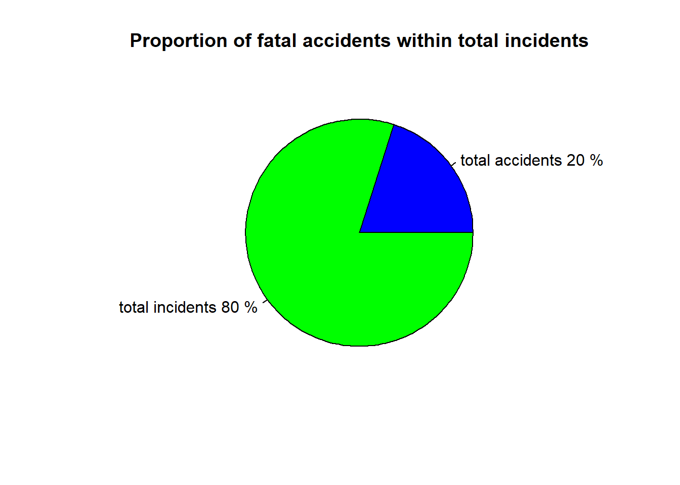
- Out of the total incidents only 20% fatal accidents happened from 1985 to 2014
9 TREND ANALYSIS
Incidents
Code
#trend analysis
library(ggplot2)
library(plotly)
inc=ggplot(ac,aes(x=airline))+
geom_line(aes(y=incidents_85_99,
color="incidents from 1985 to 1999"),
group=1,show.legend = T)+
geom_line(aes(y=incidents_00_14,
color="incidents from 2000 to 2014"),group=1,
show.legend = T)+
theme_bw()+
theme(axis.text.x = element_text(size = 8,hjust=1,angle=90))+
theme(legend.position="bottom")+
labs(colour="",
title = "Incident Trend Analysis Over Time Per Airline",
y="Incidents",x="Airlines")
ggplotly(inc)Observation
As the years approach 2014, the number of incidents are decreasing showing a decreasing trend
Fatal Accidents
Code
fa=ggplot(ac,aes(x=airline))+
geom_line(aes(y=fatal_accidents_85_99,
color="fatal accidents from 1985 to 1999"),
group=1,show.legend = T)+
geom_line(aes(y=fatal_accidents_00_14,
color="fatal accidents from 2000 to 2014"),group=1,
show.legend = T)+
theme_bw()+
theme(axis.text.x = element_text(size = 8,hjust=1,angle=90))+
theme(legend.position="bottom")+
labs(colour="",
title = "Fatal Accidents Trend Analysis Over Time Per Airline",
y="Fatal Accidents",x="Airlines")
ggplotly(fa)Observation
Decreasing trend in the number of fatal accidents
Fatalities
Code
fat=ggplot(ac,aes(x=airline))+
geom_line(aes(y=fatalities_85_99,
color="fatalities from 1985 to 1999"),
group=1,show.legend = T)+
geom_line(aes(y=fatalities_00_14,
color="fatalities from 2000 to 2014"),group=1,
show.legend = T)+
theme_minimal()+
theme(axis.text.x = element_text(size = 8,hjust=1,angle=90))+
labs(title = "Fatalities Trend Analysis Over Time Per Airline",
y="Fatalities",x="Airlines")
ggplotly(fat)Observation
From 2000 to 2014, most airlines were recording less deaths.
10 Incident Distribution Per Airline
Code
id2=ggplot(ac,aes(airline,incidents_85_99,))+
geom_segment(aes(x=airline,xend=airline,y=0,yend=incidents_85_99),
color="skyblue",size=1)+
geom_point(linewidth=2,color="black")+
coord_flip()+ theme_bw()+
theme(axis.text.y = element_text(size = 6,angle=0))+
labs(title = "Incident Distribution Per Airline",
subtitle = "1985-1999",
y="Incidents",x="Airlines")
ggplotly(id2)- only a few airlines had 0 count of incident ratios
Code
id3=ggplot(ac,aes(airline,incidents_00_14,))+
geom_segment(aes(x=airline,xend=airline,y=0,yend=incidents_00_14),
color="orange",linewidth=1, show.legend = F)+
geom_point(size=2,color="black")+
coord_flip()+ theme_bw()+
theme(axis.text.y = element_text(size = 6,angle=0))+
labs(title = "Incident Distribution Per Airline",
subtitle = "2000-2014",
y="Incidents",x="Airlines")
ggplotly(id3)Airlines such Acer Lingus have lowest ratio of incidents as compared to other airlines from 2000 to 2014.
More airline have zero count of incident ratio showing an improvement as from 1985 to 2014
Code
library(dplyr)
safe= ac %>%
dplyr::select(airline,fatal_accidents_85_99,fatal_accidents_00_14)
saf=ggplot(safe,aes(airline, fatal_accidents_85_99))+
geom_bar(aes(fill="fatal accident from 1985 to 1999"),
stat = "identity",
show.legend = T)+
geom_bar(aes(y=fatal_accidents_00_14,
fill="fatal accident from 2000 to 2014"),
stat = "identity",show.legend = T)+
theme_bw()+
theme(axis.text.x = element_text(size = 8,vjust=-0,hjust=1,angle=90))+
theme(legend.position = "bottom")+
labs(fill="",title = "Safest Airline from 1985 to 2014",
y="frequency",x="airlines")
ggplotly(saf)- Airlines such as Acer Lingus were the safest airlines since they didn’t have an accident from 1985 to 2014
11 CODE APPENDIX
Code
knitr::opts_chunk$set(echo = T, warning = F, message = F)
library(readxl)
ac = read_xlsx(file.choose())
library(janitor)
ac = clean_names(ac) #Cleaning variable names
library(knitr)
kable(colSums(is.na(ac)), caption = "Total Number of missing values in each column") #checking for missing values
anyDuplicated.default(ac)
str(ac)
kable(summary(ac), format = "pipe") #Summary Statistics
ac %>%
dplyr::select(incidents_85_99, incidents_00_14) %>%
colSums() %>%
kable()
ac %>%
dplyr::select(incidents_85_99, incidents_00_14) %>%
sum() %>%
kable()
# Fatal accidents
table(ac$fatal_accidents_85_99) %>%
kable(caption = "Count of fatal accidents by airlines from 1985 to 1999")
table(ac$fatal_accidents_00_14) %>%
  kable(caption = "Count of fatal accidents by airlines from 2000 to 2014")
library(dplyr)
ac %>%
dplyr::select(fatal_accidents_85_99, fatal_accidents_00_14) %>%
colSums()
# Total fatalities
ac %>%
dplyr::select(fatalities_85_99, fatalities_00_14) %>%
colSums()
ac %>%
dplyr::select(fatalities_85_99, fatalities_00_14) %>%
sum()
library(MASS)
sum(ac$fatal_accidents_85_99) + sum(ac$fatal_accidents_00_14) #159
kpi1 = c("total accidents", "total incidents")
values = c(159, 633)
pct = round(values/sum(values) * 100)
kpi1 = paste(kpi1, pct, "%", sep = " ")
pie(values, labels = kpi1, col = c("blue", "green"), main = "Proportion of fatal accidents within total incidents")
# trend analysis
library(ggplot2)
library(plotly)
inc = ggplot(ac, aes(x = airline)) + geom_line(aes(y = incidents_85_99, color = "incidents from 1985 to 1999"),
group = 1, show.legend = T) + geom_line(aes(y = incidents_00_14, color = "incidents from 2000 to 2014"),
group = 1, show.legend = T) + theme_bw() + theme(axis.text.x = element_text(size = 8,
hjust = 1, angle = 90)) + theme(legend.position = "bottom") + labs(colour = "",
title = "Incident Trend Analysis Over Time Per Airline", y = "Incidents", x = "Airlines")
ggplotly(inc)
fa = ggplot(ac, aes(x = airline)) + geom_line(aes(y = fatal_accidents_85_99, color = "fatal accidents from 1985 to 1999"),
group = 1, show.legend = T) + geom_line(aes(y = fatal_accidents_00_14, color = "fatal accidents from 2000 to 2014"),
group = 1, show.legend = T) + theme_bw() + theme(axis.text.x = element_text(size = 8,
hjust = 1, angle = 90)) + theme(legend.position = "bottom") + labs(colour = "",
title = "Fatal Accidents Trend Analysis Over Time Per Airline", y = "Fatal Accidents",
x = "Airlines")
ggplotly(fa)
fat = ggplot(ac, aes(x = airline)) + geom_line(aes(y = fatalities_85_99, color = "fatalities from 1985 to 1999"),
group = 1, show.legend = T) + geom_line(aes(y = fatalities_00_14, color = "fatalities from 2000 to 2014"),
group = 1, show.legend = T) + theme_minimal() + theme(axis.text.x = element_text(size = 8,
hjust = 1, angle = 90)) + labs(title = "Fatalities Trend Analysis Over Time Per Airline",
y = "Fatalities", x = "Airlines")
ggplotly(fat)
id2 = ggplot(ac, aes(airline, incidents_85_99, )) + geom_segment(aes(x = airline,
xend = airline, y = 0, yend = incidents_85_99), color = "skyblue", size = 1) +
geom_point(linewidth = 2, color = "black") + coord_flip() + theme_bw() + theme(axis.text.y = element_text(size = 6,
angle = 0)) + labs(title = "Incident Distribution Per Airline", subtitle = "1985-1999",
y = "Incidents", x = "Airlines")
ggplotly(id2)
id3 = ggplot(ac, aes(airline, incidents_00_14, )) + geom_segment(aes(x = airline,
xend = airline, y = 0, yend = incidents_00_14), color = "orange", linewidth = 1,
show.legend = F) + geom_point(size = 2, color = "black") + coord_flip() + theme_bw() +
theme(axis.text.y = element_text(size = 6, angle = 0)) + labs(title = "Incident Distribution Per Airline",
subtitle = "2000-2014", y = "Incidents", x = "Airlines")
ggplotly(id3)
library(dplyr)
safe = ac %>%
dplyr::select(airline, fatal_accidents_85_99, fatal_accidents_00_14)
saf = ggplot(safe, aes(airline, fatal_accidents_85_99)) + geom_bar(aes(fill = "fatal accident from 1985 to 1999"),
stat = "identity", show.legend = T) + geom_bar(aes(y = fatal_accidents_00_14,
fill = "fatal accident from 2000 to 2014"), stat = "identity", show.legend = T) +
theme_bw() + theme(axis.text.x = element_text(size = 8, vjust = -0, hjust = 1,
angle = 90)) + theme(legend.position = "bottom") + labs(fill = "", title = "Safest Airline from 1985 to 2014",
y = "frequency", x = "airlines")
ggplotly(saf)